Avid computer vision readers know that lately, transformer models have become all the hype as they show a convenient way of training deep learning models without the sequential models like RNNs or making use of the convoluted ways of CNNs (pun-intended). As I treaded down this path, I realized there were a lot of moving parts to transformers that are harder to streamline unlike CNNs. I am making this post for the learners as well as myself to refer back to for clarification. Here, I want to explore why do the transformers and specifically attention, which is the main component of the model work so well in a wide range of problems.

One of the earliest adaptations of the attention module was it’s use in natural-language processing for sentence translation. Attention module was used with RNNs for use in sequence to sequence model where one input is passed in one at a time, generates a hidden state and the second input is passed in along with the previous hidden state to generate the next vector. With the attention module, researchers realized that attention module can be used by itself instead of in a RNN or LSTM network. Hence, came the transformers networks that take the input simultaneously, much like CNNs and are faster than RNNs since they are sequential in their processing of the input. Since, this blog is focused on computer vision techniques, the article will discuss techniques applicable on images data.

Transformers:

A standard transformer network consists of an encoder-decoder architecture. The input is passed into the encoder and it passes through several self-attention and dense layers and outputs vectors. The decoder network takes in the target along with the output of the encoder and processes the inputs by passing them through self-attention and dense layer. The main architecture of the encoder-decoder is depicted in the image below.

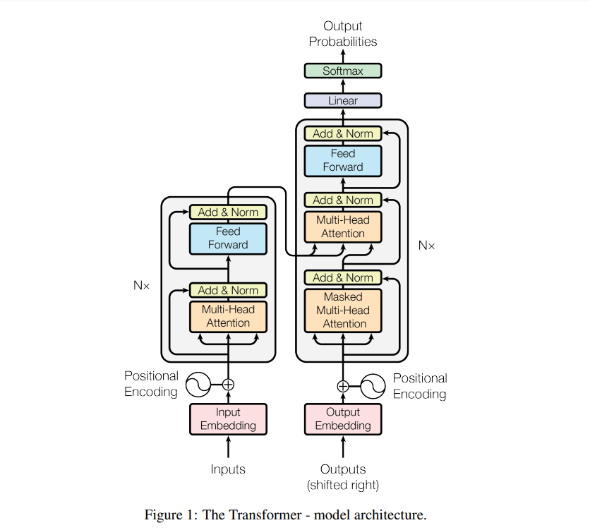Credit: Attention is All You Need by Vaswani et al.

Embeddings and Encodings of the Input

For image processing through transformers, the image is divided into a fixed number of patches, depending on the dataset and image original sizes. Each patch is then vectorized and mapped to D dimensions with a trainable linear projection in the form of a linear layer. The W matrix and b of this linear layer are learnable parameters. Next step is to add the positional encodings about the patches as it corresponds to their position in the image. Since the model does not have spatial processing like RNNs or CNNs do, we need to pass in the positional encodings of the inputs. In the original attention paper, the researchers were dealing with NLP so they used sinusoidal functions to create positional encodings for words in a sentence. In the case of computer vision, since we are dealing with image patches, something as simple as numbering each patch one by one should accomplish the task. However, the researchers performed ablation studies on different ways of encoding spatial information. They tried experiments with no embeddings, 1-dimensional embeddings, 2-dimensional embeddings by considering patches as a part of a grid. The performance of the model was poor when no positional embedding was added to the input but the performance was much better when there is a positional embedding present, regardless of the type of the embedding. After adding the embedding, the input is ready to be passed into a self-attention layer, the details of which are described below.

Self-Attention:

The idea of self-attention stemmed from the attention module used in the RNNs. The attention module can be described as a function that maps a query and a set of key-value pairs to an output, where all three query, key, and value are vectors Vaswani et al.. The output of the attention module is a weighted sum of the values, where the weights are calculated by a compatibility function of the query with the corresponding key. In simpler terms, one query vector interacts with all the keys and determines which value should be weighted more than the others for that certain query. This will be explained more in detail. The following function summarizes the attention module:

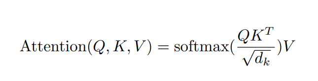
The above equation summarizes the self-attention part of the transformer. The function computes the connection or relation of every input to every other input. The following paragraphs breakdown all the calculations included in the self-attention layer. First step in self-attention layer is to use the input to get the key, value and query vectors.

The W matrices for the key, value and query vectors are what we optimize with transformer networks. They are initialized to random weights and we optimize them through the training of the transformer network. Next, we calculate the relationship of one query vector to all the key vectors. Query can be considered a target and each query tries to calculate to relationship with all the input keys. This connections is depicted in the equation of the alpha vector.

For an input ranging from 1 to m x-vectors, the alpha vectors are calculated using just one query and keys from all the m input vectors. The elements of alpha~1 indicate how well the query vector~1 is aligned with all the keys of the inputs. So, the alpha vector of any input vector x, it takes in all the key vectors as a matrix and one query vector. The matrix-vector multiplication is then passed into the softmax function.

Once the alpha vector has been calculated, we calculate the context vector which holds the relevant information about the values of the input keys. It is the weighted average of the value vectors of all the x inputs. The context vector takes the alpha for one input value and takes all the values of the input x vectors.

The context vector shows mapping of a single query to all the keys and values functions and then, the training of the model optimizes the relationship between a certain query~j with all the keys and values of the input. The same way, alpha~2~ is calculated using the second query vector and all the keys of the input vectors x. Then, the context vector is calculated using alpha vector for the input x and all the values. The following equation summarizes the context vector relationship with query, key, and value vectors.

This is the weighted sum of the value vectors and the weight assigned to each value is computed by the compatibility function shown above. This is because one context vectors depends on all the keys and values vectors from the inputs. The parameters to be learned from the self-attention layers are W_Q, W_K, W-V.

This post summarizes the self-attention module and how one query interacts with all the keys and values to determine how much weight should be placed on each value to get the desired result. Next post will detail the use of self-attention module in Vision Transformers.